Solving Data Science tasks with Greenplum DB

Until 2016, the terms “data science” and “data mining” usually meant the use of the Hadoop ecosystem. But the game changed about two years ago. Many enterprises have faced the fact that the Hadoop stack is too heavy to use entirely for enterprise tasks.

In addition to the Hadoop distribution itself (with about 20+ separated components), you must also take care of the necessary operation tasks, components version compatibility, etc. Moreover, to use your cluster for business tasks, you will need developers with knowledge of the specifics of Hadoop development, and there are not many of these professionals on the market now. All of these are well-known problems of using Hadoop in enterprise. Maybe that’s why there is no more Hadoop reference neither on the Cloudera landing page nor on the Strata Big Data conference. Nowadays, Hadoop is not used as a single data machine anymore – only some of its components (like Kafka, Spark, or NiFi) are still used in new production environments.

On the contrary, traditional RDBMSs are more understandable to businesses, cheaper to maintain and require less development costs. Modern massive parallel processing (MPP) databases are in no way inferior to Hadoop in their ability to parallelize tasks and scale. But is it possible to use MPP RDMS for typical Hadoop cases – Data Science and Data Mining?

In this article I will use my favorite cluster technology – Greenplum (GP) – to show how traditional big data tasks can be solved using RDBMS. GP is a flexible open-source MPP RDBMS based on PostgreSQL that provides fully compatible ANSI SQL access to your data. Greenplum uses multiple (from two to hundreds) servers to provide scalability and high-availability functionality. My demo Greenplum cluster for this article consists of three VMs: mdw (master node), sdw1 and sdw2 (segment nodes). Each segment node contains two logical segments.

This article consists of four parts:

1. Basics
   Here we will find out what a typical User Defined Function is and how it can be executed in parallel.
2. Security
   We will talk about user permissions and function isolation when running UDFs.
3. MapReduce
   We will create a simple Python MapReduce-like program using an AGGREGATE function.
4. Near-real-world example
   We will take one of the typical data science tasks – text sentiment analysis – and try to solve it within Greenplum DB.

Basics

Most data science and data mining tasks are solved with two environments: R and Python. These two programming languages are de facto standard for data tasks. They both have big amounts of additional modules, including natural language processing, voice recognition, machine learning, etc. Both Python and R are parallelized in a Hadoop cluster using PySpark or SparkR functionality, so your code is executed on every server in the cluster (in general).

RDBMSs provide their own way to execute a user’s code, it’s called User Defined Functions, or UDF. UDF is a function that a developer creates using different programming languages and that users can access in SQL queries in the RDBMS. As for Greenplum, the following languages are supported:

• Python
• R
• Java
• Perl
• SQL

Moreover, you can add support of other languages by using the CREATE LANGUAGE statement and assigning necessary functions.
In this article I will use Python, but the algorithm is pretty much the same for any other language.

Let’s prepare some example data to play with:

-- Create the table with just one text field
create table urls
(
url_path text
)
-- I want this table to be column-oriented
with (appendonly=true, orientation=column)
/* I want this table to be spread across Greenplum 
cluster based on the column's values */
distributed by (url_path);

-- Insert some urls into the table 
insert into urls values
('https://greenplum.org/blog/'),
('https://github.com/greenplum-db/gpdb'),
('https://dwhsys.com/author/'),
('https://web.telegram.org/#'),
('http://help.statsbot.co/how-to-connect-database-to-statsbot'),
('https://medium.com/tensorist/tagged/machine-learning'),
('http://185.193.143.202:45914/#/notebook/2DB7UZ74B');

Now lets create a simple UDF using the Python language that parses the urls from the given table and outputs the hostname (netlocation):

-- Create the function and set the input type
create or replace function extract_host_simple(url text)
-- Define the output type
returns text
as $$
-- Here is where the Python code starts
import urlparse
return urlparse.urlparse(url).netloc
$$
language plpythonu;

-- Now let's try our function:
select extract_host_simple(url_path) from urls;

And the result will be:

extract_host_simple
greenplum.org
dwhsys.com
185.193.143.202:45914
medium.com
github.com
web.telegram.org
help.statsbot.co

Simple, isn’t it?
Now let’s make our UDF a little more complicated. Let’s add to the output the information about the host that this UDF was run at.

drop function extract_host(url text);
create or replace function extract_host(url text) returns text  
as $$
import urlparse
import socket
return urlparse.urlparse(url).netloc + '. This row was generated on host ' + socket.gethostname()
$$
language plpythonu;

select extract_host(url_path) from urls;

The result will be:

extract_host
greenplum.org. This row was generated on host sdw1
185.193.143.202:45914. This row was generated on host sdw1
dwhsys.com. This row was generated on host sdw1
medium.com. This row was generated on host sdw1
github.com. This row was generated on host sdw2
web.telegram.org. This row was generated on host sdw2
help.statsbot.co. This row was generated on host sdw2

This example shows that our UDF is executed in parallel on every cluster segment host based on row location.

Security

You might notice a problem: if you allow database users to create a UDF, they can possibly:

• badly corrupt all your database by escaping to shell
• grab all the resources of the DBMS cluster
• perform many other bad things

For example, let’s create a UDF that will be a DB-killer. It will totally delete all of the existing data either on the master server or on every segment server of your Greenplum cluster based on the way of its execution. Every user that has access to the PLPython language can run it.
We assume that the /data directory is the directory where the DB files are stored.
WARNING! Do not run this UDF in your database!

create or replace function catharsis()  
as $$
import os
return os.system('rm -rf /data')
$$
language plpythonu;

To secure your database and to limit user’s UDF resources you can use docker containers to run UDF. In this case all user’s actions will be performed inside a container that is limited by memory, CPU and network resources. Moreover, if a user tries to corrupt the container, the DB will not be affected.
Initial setup of the PL/Container for the Pivotal non-open source version of GP is explained in the corresponding article in Greenplum’s blog. Open-source PL/Container installation is pretty much the same, except the package install and image creation, so let’s go ahead to its usage.
In the case of using PL/Container, our DB-killer UDF will look like this:

create or replace function catharsis()  
returns text
as $$
/* This is the name of the Docker image that
will be used for the containers */
# container: plc_py
import os
return os.system('rm -rf /data')
$$
-- We restrict our users from using plpythonu PL
-- and allow them to run only plcontainer PL
language plcontainer;

This UDF is absolutely safe to run:

• After the next restart of the container (which is done automatically after a user’s session is closed) the environment will be ready again.
• Other users’ containers will not be affected.
• The user that ran the DB-killer will understand that he has broken his container and hopefully will review his code. True catharsis.

Now lets run our extract_host function in the container environment. Just two small changes make our function run inside Docker:

drop function extract_host(url text);
create or replace function extract_host(url text) returns text  
as $$
# container: plc_py
import urlparse
import socket
return urlparse.urlparse(url).netloc + '. This row was generated on host ' + socket.gethostname()
$$
language plcontainer;

And now the result will show us that the Python code was executed inside a container:

extract_host
github.com. This row was generated on host 2c12c388fcae
web.telegram.org. This row was generated on host 2c12c388fcae
help.statsbot.co. This row was generated on host 2c12c388fcae
medium.com. This row was generated on host b844ca9eaf5a
greenplum.org. This row was generated on host bef8be6e769d
dwhsys.com. This row was generated on host bef8be6e769d
185.193.143.202:45914. This row was generated on host bef8be6e769d

Notice that there are three different containers used in running this UDF. These containers were run on a two-segement host. If I had more data in the table, four containers (because I have four segments in my DB) would be used.

MapReduce

Now we have all the necessary instruments to create a simple MapReduce task using UDFs. Our MapReduce function will be a regular summary aggregative function that will sum up all the values of the given column. The function will consist of three parts:

• Segment function (map function) – this function will be executed locally on every segment in the cluster with every row.
• Master function (reduce function) – this function will be executed on master segment. It will take as parameters every segment’s function results
• Final function – this function will take the master’s function result and apply some transformations to it. In my example, this function will multiply the result by 1 (do nothing).

-- The segment function
CREATE OR REPLACE FUNCTION segment_sfunc(int1 int, int2 int) 
  RETURNS int
   AS $$
   # container: plc_py
    var1=int1
    var2=int2
    return var1 +  var2
   $$
   LANGUAGE plcontainer
 /* This tells the optimizer that the function returns
 the same result on the same input and thus the result may
 be cached */ 
   IMMUTABLE
   RETURNS NULL ON NULL INPUT;

-- The master function   
CREATE OR REPLACE FUNCTION master_prefunc(int1 int, int2 int) 
  RETURNS int
   AS $$
   # container: plc_py
    var1=int1
    var2=int2
    return   var1 + var2
   $$
   LANGUAGE plcontainer
   IMMUTABLE
   RETURNS NULL ON NULL INPUT;

/* The final function. Note that I used SQL
for the final function and plcontainer
for segment and master functions. You can
combine different UDF languages in one
aggregate function */
CREATE OR REPLACE FUNCTION final_func(int)
  RETURNS int
   AS $$
   select $1*1
   $$
   LANGUAGE SQL
   IMMUTABLE
   RETURNS NULL ON NULL INPUT;

Now we can combine all three functions in the aggregation function:

   
  DROP    AGGREGATE agg_func(int);
  CREATE AGGREGATE agg_func(int) (
   SFUNC = segment_sfunc,
-- This is the type of the intermediate result
   STYPE = int,
   FINALFUNC = final_func,
   PREFUNC = master_prefunc,
   INITCOND = 0 );

Running this function will give the same result as a sum() function:

 
select agg_func(1), sum(1) from urls;

agg_func	sum
7	7

And the execution plan of the function will show that the function was executed firstly on segments, and secondly on the master host:

 
explain select agg_func(1) from urls;

query_plan
Aggregate (cost=0.00..431.00 rows=1 width=4) -> Gather Motion 4:1 (slice1; segments: 4) (cost=0.00..431.00 rows=1 width=4) —-> Aggregate (cost=0.00..431.00 rows=1 width=4) ——-> Table Scan on urls (cost=0.00..431.00 rows=2 width=1)

You can use aggregate functions for solving typical MapReduce tasks using your MPP cluster Database – text mining, computing stats, and of course for counting words 🙂 A user that will use your code may not even know that there is a Python code written and Python libraries used – all he needs to operate is SQL – one of the “cheapest” programming languages.

Near-real-world example

For proving my assumption that a typical data science task can be solved using traditional enterprise MPP RDBMS and some UDFs, I took one of the natural language processing examples published on Medium – Sentiment analysis for Yelp review classification. This great example uses Python, NLTK, NumPy, scikit-learn and Pandas to build a basic text classifier model that predicts whether a user liked a local business or not, based on their review on Yelp.
Basically the task consists of the following subtasks:

1. Preparing data
2. Getting base metrics about the Yelp reviews using pandas
3. Exploring the dataset using Seaborn and Matplotlib visualizing tools
4. Choosing independent and dependent variables
5. Review text preprocessing: removing the stopwords, punctuation, etc.
6. Training the model
7. Testing the model

For simplicity, I will use pure Python UDFs without the PL/Container extension and AGGREGATE functions. In real enterprise usage, as we learned before, these two modifications of the UDFs will significantly improve performance, security, and operationality of the code.

1. Preparing data

For this example we need sample Yelp data, which is presented by the corresponding CSV file to our database. This can be easily done with a Greenplum external table:

-- Dropping and creating the external table
drop external table if exists yelp_ext;
create external web  table yelp_ext
(business_id text,
date date,
review_id text,
stars int,
text text,
type text,
user_id text,
cool int,
useful int,
funny int
)
-- I placed the csv on the master host
EXECUTE 'cat /opt/yelp.csv' ON MASTER
 FORMAT 'CSV' ( DELIMITER ',' HEADER );

-- Dropping and creating the usual Greenplum compressed columnar table
drop table if exists yelp;
create table yelp (like yelp_ext)
with (appendonly=true, orientation=column, compresstype=zlib, compresslevel=7);
-- Copying the data from the csv file to the DB table
insert into yelp select * from yelp_ext;

2.Getting base metrics

Now, when the data is loaded into the database as a typical table, we can get some statistics from the Pandas library.
Please note that this function will not be run in parallel, it will be executed only on master host.

drop function if exists describe_yelp();
create or replace function describe_yelp(
-- We need to specify output fields and types
OUT stats text,
OUT stars numeric,
OUT cool numeric,
OUT useful numeric,
OUT funny numeric,
/* Comparing the original medium article,
I added review text length to the
description dataset - this will give us some basic
info about the review text */
OUT txt_length numeric)
returns setof record
as $$
import pandas as pd
import numpy as np
import nltk
from nltk.corpus import stopwords
-- We need to specify the order of the columns
yelp=pd.DataFrame.from_records(plpy.execute('select * from yelp'))[['stars','cool','useful','funny','text']]
-- Adding the text length value to the dataset
yelp['txt_length'] = yelp['text'].apply(len)
/* The simplest way to return the result table to the 
database is by using NumPy records */
return yelp.describe().to_records()      
$$
language plpythonu;

select * from describe_yelp();

This will give us base stats about the stars and review text length:

stats	stars	cool	useful	funny	txt_length
count	10000.0	10000.0	10000.0	10000.0	10000.0
mean	3.7775	0.8768	1.4093	0.7013	710.7541
std	1.2146362764747367	2.0678610603559644	2.3366470640535755	1.907941910602475	617.4245665202545
min	1.0	0.0	0.0	0.0	1.0
25%	3.0	0.0	0.0	0.0	294.0
50%	4.0	0.0	1.0	0.0	541.5
75%	5.0	1.0	2.0	1.0	930.0
max	5.0	77.0	76.0	57.0	4997.0

3. Exploring the dataset using the Seaborn and Matplotlib visualizing tools

Basically, a database is not a good place to visualize data – there are a lot of great additional software that can visualize your in-database data using SQL access – BI tools, ad-hoc analytic tools, SQL IDE, etc. But, if we are following the Medium article in its entirety, we should use the same visualization tools – Matplotlib and Seaborn.
Let me explain a crazy thing I am going to do in the next UDF:

1. I will build a Seaborn FacetGrid chart.
2. I will place it in a memory buffer.
3. I will encode it using Base64.
4. I will construct an html code containing the image.
5. I will get the html code to Apache Zeppelin using the SQL interpreter (Ipython Notebook SQL kernel analog).
6. Zeppelin will construct the image from the html-code and print it in the SQL output cell.

Once again, there are a lot of other visualization tools that you should prefer while visualizing your relational data – this is just a crazy PoC:

drop function if exists facet_grid_html_img();
create or replace function facet_grid_html_img()
returns text
as $$
import pandas as pd
import numpy as np
import matplotlib
-- We dont want to use the $DISPLAY variable
matplotlib.use('Agg')
import matplotlib.pyplot as plt
import seaborn as sns
import nltk
import io
from Tkinter import *
from nltk.corpus import stopwords

yelp=pd.DataFrame.from_records(plpy.execute('select * from yelp'))[['stars','cool','useful','funny','text']]
yelp['txt_length'] = yelp['text'].apply(len)
g = sns.FacetGrid(data=yelp, col='stars')
g.map(plt.hist, 'txt_length', bins=50)
buf = io.BytesIO()
g.savefig(buf, format='png')
buf.seek(0)
data_uri= buf.read().encode('base64')
img_tag = '%html <img src="image/png;base64,{0}">'.format(data_uri)
return img_tag
$$
language plpythonu;

select * from facet_grid_html_img();

And here is the rendered image:

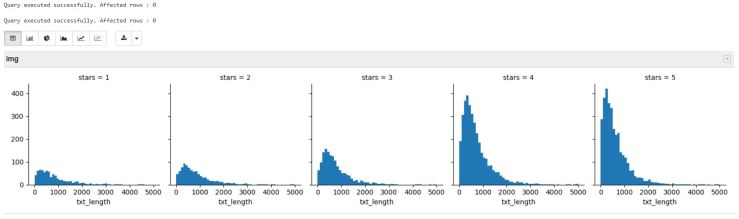
This grid shows us that review text length is similar in all star ratings, and that there are more 4-star and 5-star ratings in the dataset than others.
The next step in the original article is to create a boxplot of the text length for each star rating. We will do it absolutely the same, and will get the plot:

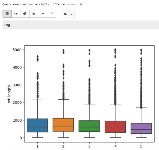
This plot proves that the review length for the first look isn’t a good way to predict rating.

The next step is grouping the dataset by star rating, and seeing if it is possible to find a correlation between cool, useful, and funny features using the corr() pandas method:

...
stars = yelp.groupby('stars').mean()
return stars.corr().to_records()
...

Let’s build the heatmap using the same way as for the boxplot:

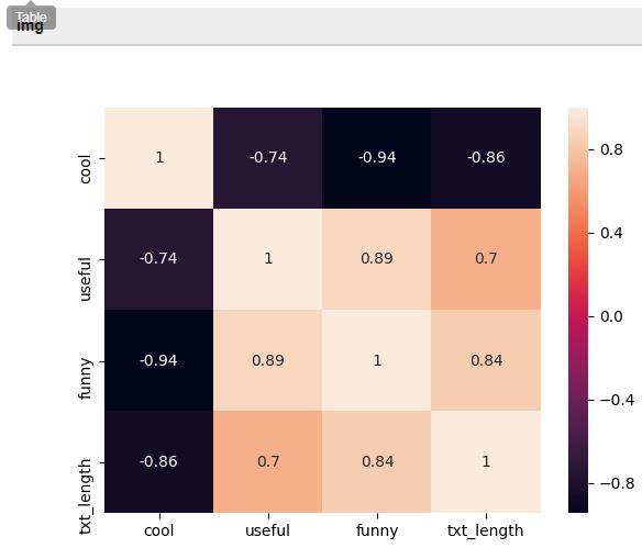
The map shows that funny is strongly correlated with useful, and useful seems strongly correlated with text length, and that there is a negative correlation between cool and the other three features.

4. Choosing independent and dependent variables

Now we need to leave only 1-star and 5-star reviews and to assign the variables:

...
-- Get rid of 2,3,4-star reviews
yelp_class = yelp[(yelp['stars'] == 1) | (yelp['stars'] == 5)]
yelp_class.shape
-- Assigning the variables
X = yelp_class['text']
y = yelp_class['stars']
...

5. Review text preprocessing

To use the classification algorithm we need to remove stop words and punctuation. The author of the original article creates a function that removes punctuation, stopwords, and returns a list of the remaining words, or tokens, that the classification algorithm will use. We can check how it works inside a UDF by creating a simple text-returning UDF:

create or replace function stopword_check()
returns text
as $$

import pandas as pd
import numpy as np
import nltk
import string
from nltk.corpus import stopwords

def text_process(text):
    '''
    Takes in a string of text, then performs the following:
    1. Remove all punctuation
    2. Remove all stopwords
    3. Return the cleaned text as a list of words
    '''
    nopunc = [char for char in text if char not in string.punctuation]
    nopunc = ''.join(nopunc)
    
    return [word for word in nopunc.split() if word.lower() not in stopwords.words('english')]

sample_text = "Hey there! This is a sample review, which happens to contain punctuations."
return(text_process(sample_text))
$$
language plpythonu;

select * from class();

And it works perfectly:

class
[‘Hey’, ‘sample’, ‘review’, ‘happens’, ‘contain’, ‘punctuations’]

6. Training the model

Now we are ready to train our model. All in one, the model-training UDF will look like this:

create or replace function yelp_train_model()
returns text
as $$

import pandas as pd
import numpy as np
import nltk
import string
import sklearn
import socket
from nltk.corpus import stopwords
from sklearn.feature_extraction.text import CountVectorizer
from sklearn.model_selection import train_test_split
from sklearn.naive_bayes import MultinomialNB
from sklearn.externals import joblib
-- As we want to reuse our model in the future, we will dump it to file on
-- masters filesystem
model_file='/tmp/model_file.sav'
-- We also need to dump the vocabulary to use it in the future
vocab_file='/tmp/vocab_file.sav'

def text_process(text):
    nopunc = [char for char in text if char not in string.punctuation]
    nopunc = ''.join(nopunc) 
    return [word for word in nopunc.split() if word.lower() not in stopwords.words('english')]

yelp=pd.DataFrame.from_records(plpy.execute('select * from yelp'))[['stars','cool','useful','funny','text']]
yelp['txt_length'] = yelp['text'].apply(len)


yelp_class = yelp[(yelp['stars'] == 1) | (yelp['stars'] == 5)]
yelp_class.shape
X = yelp_class['text']
y = yelp_class['stars']
bow_transformer = CountVectorizer(analyzer=text_process).fit(X)
X = bow_transformer.transform(X)
X_train, X_test, y_train, y_test = train_test_split(X, y, test_size=0.3, random_state=101)
nb = MultinomialNB()
-- Training the model
nb.fit(X_train, y_train)
-- Dumping the vocabulary and the model
joblib.dump(bow_transformer.vocabulary_,vocab_file,compress=9)
joblib.dump(nb,model_file, compress=9) 

-- Some info in the output
return('Model was trained and saved to ' + model_file + ' on host ' + socket.gethostname())  
$$
language plpythonu;

select * from yelp_train_model();

yelp_train_model
Model was trained and saved to /tmp/model_file.sav on host mdw

7. Testing the model

Here is the moment of truth: now we can test our created model on database data. After distributing the vocabulary and model files across all machines in a cluster we need to create a UDF for executing the model that will be run in parallel using all servers in the cluster:

-- The function takes review text as an argument 
-- And returns its predicted rating
create or replace function yelp_test_model(review text)
returns int
as $$
import string
from nltk.corpus import stopwords
from sklearn.feature_extraction.text import CountVectorizer
from sklearn.naive_bayes import MultinomialNB
from sklearn.externals import joblib
vocab_file='/tmp/vocab_file.sav'
model_file='/tmp/model_file.sav'

def text_process(text):
    nopunc = [char for char in text if char not in string.punctuation]
    nopunc = ''.join(nopunc)
    return [word for word in nopunc.split() if word.lower() not in stopwords.words('english')]
-- Importing the vocabulary and the model
nb=joblib.load(model_file)
vocabulary=joblib.load(vocab_file)

r_review = CountVectorizer(analyzer=text_process,vocabulary=vocabulary).transform([review])
--
return(nb.predict(r_review)[0])
$$
language plpythonu;

-- Running the function to compare the real result
-- with the predicted value for ten random reviews
select yelp_test_model(text),stars from yelp limit 10

yelp_test_model	stars
5	4
5	4
5	5
5	4
5	5
5	4
5	4
1	1
1	1
5	4

The result shows us that that our model works. It works not as well as it could because the model is more biased towards positive reviews compared to negative (the author of the original article notices it), so some of the negative reviews will be marked as positive, but the concept is working and further model optimizations can be done.
As you might notice, our model UDF is not optimized for processing large amounts of data – the Python code is executed one time per one row, so every import of Python modules and export of data files will result in huge overhead.
The PL/Python extension provides some instruments to avoid this. Here’s how the UDF will look with some of the optimizations:

create or replace function yelp_test_model(review text)
returns int
as $$
/* We are using a Global Directory (GD) list to store previously imported modules
so every module will be imported only once per database session.
GD is shared across all functions in one database session */
if 'string' not in GD:
    import string
    GD['string']=string
string=GD['string']

if 'stopwords' not in GD:
    from nltk.corpus import stopwords
    GD['stopwords']=stopwords
stopwords=GD['stopwords']

if 'CountVectorizer' not in GD:
    from sklearn.feature_extraction.text import CountVectorizer
    GD['CountVectorizer']=CountVectorizer
CountVectorizer=GD['CountVectorizer']

if 'MultinomialNB' not in GD:
    from sklearn.naive_bayes import MultinomialNB
    GD['MultinomialNB']=MultinomialNB
MultinomialNB=GD['MultinomialNB']

if 'joblib' not in GD:
    from sklearn.externals import joblib
    GD['joblib']=joblib
joblib=GD['joblib']

vocab_file='/tmp/vocab_file.sav'
model_file='/tmp/model_file.sav'

/* The same approach works well with model and vocabulary
files - they will be read from disk just once */ 

if 'model' not in GD:
    model=joblib.load(model_file)
    GD['model']=model
model=GD['model']

if 'vocabulary' not in GD:
    vocabulary=joblib.load(vocab_file)
    GD['vocabulary']=vocabulary
vocabulary=GD['vocabulary']

def text_process(text):
    nopunc = [char for char in text if char not in string.punctuation]
    nopunc = ''.join(nopunc)
    return [word for word in nopunc.split() if word.lower() not in stopwords.words('english')]

r_review = CountVectorizer(analyzer=text_process,vocabulary=vocabulary).transform([review])

return(model.predict(r_review)[0])
$$
language plpythonu;

Other optimizations can also be done: the function text_process can be moved to a module and stored in GD, the UDF can be run once per all data on a segment, the vocabulary and the model data can be stored not in files but as a byte object inside a table, etc.

This exercise showed us that a traditional MPP database can be used for solving typical data science and data mining tasks, but, compared to a Hadoop cluster and standalone Python installation, our version:

• Provides SQL access to developed models and algorithms (every DB user can use our model like “select yelp_test_model(‘Some text’)”)
• Can be easily integrated with ETL/ELT and BI tools
• Can split model execution to multiple servers without rewriting Python code

Onthe other hand, using MPP as an execution engine requires you to understand the principles of MPP and take a little bit different approach in storing data.

In conclusion, I suggest you take a look at the potential of MPP databases in data science tasks. Greenplum DB is an open-source and free-to-use product that perfectly fits an in-database analytics approach.

Feel free to contact me for any Greenplum-related questions, consulting, integrations, and support.